HLO Visualizer: Learn XLA HLO by Exploring It
- EN
- ZH-CN
Table of Contents
When working with JAX on TPU, you eventually need to read HLO. You want to know what a computation became after compilation, why extra copies appeared, or what is inside a fusion. The answers start with a compiler-generated text file.
Instructions pack together shapes, layouts, tiling, memory spaces, and references to other computations.
I built HLO Visualizer to make that easier. It turns HLO text into an explorable graph, with explanations of the instruction you select, piece by piece.
#
From seeing the graph to understanding an instruction
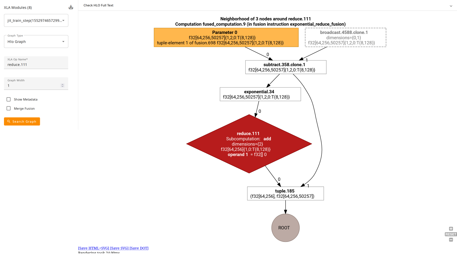
There is already an official HLO visualization tool: XProf’s Graph Viewer. It lets you explore an operation’s neighborhood, expand or collapse fusions, and connect the graph to profiling data. That is useful when you have identified an expensive operation and want to understand its dependencies. The official documentation describes this workflow.
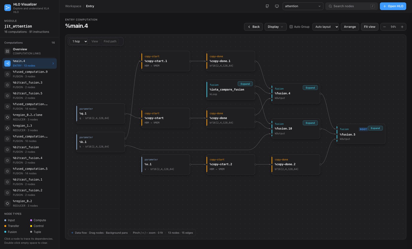
HLO Visualizer puts the graph and the explanation in one interface. Nodes distinguish inputs, computation, transfers, and control flow. Select one to trace dependencies, inspect its original HLO, and navigate to the computations it references.
XProf connects HLO to measured performance. HLO Visualizer starts with a piece of HLO text you want to understand.
#
Put the tutorial beside the instruction
Google DeepMind’s How to Scale Your Model has a useful introduction, How to read an XLA op. It explains names, types, layouts, memory locations, and operands through a fusion example. OpenXLA’s Operation semantics is the reference for precise operation behavior.
The next step is applying those rules to your own program.
Consider this simplified instruction:
%x = bf16[128,128]{1,0:T(8,128)(2,1)S(1)} parameter(0)
It contains several layers of information:
%xnames the instruction’s result.bf16[128,128]gives the logical type and shape.1,0is the minor-to-major dimension order.T(8,128)(2,1)describes two levels of physical tiling.S(1)means VMEM in these TPU examples.parameter(0)declares input 0 of the current computation.
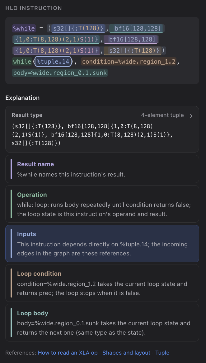
The inspector breaks the original instruction into colored segments and explains its name, operation, operands, and attributes. Expand the type to inspect shape, dimension order, tiling, and memory space separately. Tuple elements can be explored individually too.
#
Draw the TPU layout
Layout is an important part of HLO. Logical shape and physical storage layout describe different things. A 128 × 128 array can be split into tiles, with another level of tiling inside each tile. OpenXLA’s Shapes and layout and Tiled layout document the representation.
For the common TPU layout T(8,128)(2,1), HLO Visualizer draws a corner of a tile, labeling physical offsets and inner tile boundaries. The two sets of numbers become something you can see.
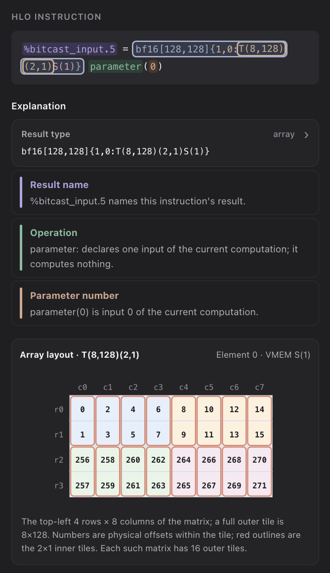
The tool also explains TPU memory locations such as HBM, VMEM, and SMEM, helping you interpret transfer instructions. Memory-space numbers depend on the backend; the explanations here use the project’s TPU v6e examples as their context.
#
Start with a small program
The bundled examples come from 21 small JAX programs compiled on TPU v6e, each with HLO before and after optimization. Try attention for inputs and fusions, fori_matmul for loops, or gather_scatter for indexing operations.
Open an example, enter its entry computation from the sidebar, and select a node. Inspect its inputs and result type, then explore a computation referenced by a fusion or while. Switch between Before and After in Examples to inspect how compilation changes the graph.
To explore your own code, export HLO through JAX’s lowering and compilation interfaces:
import jax
import jax.numpy as jnp

def f(x, w):
    return jax.nn.relu(x @ w)

x = jnp.ones((128, 128), dtype=jnp.bfloat16)
w = jnp.ones((128, 128), dtype=jnp.bfloat16)
lowered = jax.jit(f).lower(x, w)

# HLO before optimization
print(lowered.as_text(dialect="hlo"))

# Compiled HLO; layouts and memory spaces depend on the backend
print(lowered.compile().as_text())
Copy either output and paste it through Open HLO. HLO text from XLA’s --xla_dump_to works too.
I want someone learning HLO for the first time to be able to connect the syntax to a small, real program. Open the graph, select an instruction, and follow the data.
Try HLO Visualizer. If it helps you understand your HLO, a star on GitHub is welcome. Please open an issue for instructions that are unclear or do not parse correctly.